​经过了前面一段的铺垫学习,总算走到了这次的目标:利用 TensorFlow 实现 Attention-based LSTM 来做 Text Classification,主要是在前面一篇文章讲的 TensorFlow 提供的 RNN(GRU) Model 上面添加 Attention Mechanism,注意力模型的实现上,我主要参考了 Attention-Based Bidirectional Long Short-Term Memory Networks for Relation Classification 这篇论文。

原理

上面那篇文章和我想做的东西是非常类似的,唯二的两个区别是:

一、它使用了一个双向 LSTM 来解决长句子后半部信息丢失的问题,我只是用了单向的 LSTM

二、它做的是 Relation Classification,而我是 Text Classification。

Attention

论文中 Attention 的公式如下:

Attention Principles

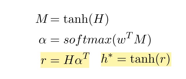
T:文档的长度,在我们的代码里被设置为 MAX_DOCUMENT_SIZE

H:每个 LSTM 的 output 的集合,即 [h1, h2, … , hT],维度:(Embedding Size,T)

α:注意力向量,也就是一个 h 的权重分布向量,我们通过 W^T^H,希望能够模型学习得到 Weight,进一步得到 α,维度:(1,T)

r:加权后的 H,维度:(Embedding Size,1)

h*:最后的输出,添加一层 tanh ,把值变换到[-1, 1]区间,维度:(Embedding Size,T)

Classifying

Classifying

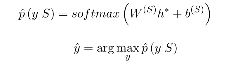
通过 Softmax 函数我们得到一个类别的概率向量,然后再用 argmax 函数的结果作为我们最终的分类。

Explanation

其实我们可以通过几个向量的维度窥得其中几个重要的物理意义:

  1. α 的维度和文本长度相等,注意力向量的加权的思想体现在这里。
  2. r 向量的长度和词嵌入的长度相同,可以认为是把整篇文章通过 Attention Model 变成了一个 Topic Word,随后我们通过学习 Softmax 层的 Weight 和 Bias 来找到各个 Topic Word 在词嵌入的高维空间之中对应的类别。如果能够把结果 plot 出来,应该能看到同一类别文本的 Topic Word 是相近的。

TensorFlow 实现

1
2
3
4
5
6
7
8
9
10
11
12
13
14
15
16
17
18
19
20
21
22
23
24
25
26
27
28
29
30
31
32
33
34
35
36
37
38
39
40
41
42
43
44
45
with graph.as_default():

    batch_x = tf.placeholder(tf.int32, [None, MAX_DOCUMENT_LENGTH])
    batch_y = tf.placeholder(tf.float32, [None, MAX_LABEL])
    keep_prob = tf.placeholder(tf.float32)
    
   # Embedding Var, train word embedding during the training 
    embeddings_var = tf.Variable(tf.random_uniform([n_words, EMBEDDING_SIZE], -1.0, 1.0), trainable=True)
    batch_embedded = tf.nn.embedding_lookup(embeddings_var, batch_x)
    W = tf.Variable(tf.random_normal([HIDDEN_SIZE], stddev=0.1))
    # print(batch_embedded.shape)  # (?, 256, 100)

    rnn_outputs, _ = bi_rnn(BasicLSTMCell(HIDDEN_SIZE), BasicLSTMCell(HIDDEN_SIZE),
                            inputs=batch_embedded, dtype=tf.float32)
    # Attention
    fw_outputs = rnn_outputs[0]
    # print(fw_outputs.shape)
    bw_outputs = rnn_outputs[1]
    H = fw_outputs + bw_outputs  # (batch_size, seq_len, HIDDEN_SIZE)
    M = tf.tanh(H) # M = tanh(H)  (batch_size, seq_len, HIDDEN_SIZE)
    # print(M.shape)
    # alpha (bs * sl, 1)
    alpha = tf.nn.softmax(tf.matmul(tf.reshape(M, [-1, HIDDEN_SIZE]), tf.reshape(W, [-1, 1])))
    r = tf.matmul(tf.transpose(H, [0, 2, 1]), tf.reshape(alpha, [-1, MAX_DOCUMENT_LENGTH, 1])) # supposed to be (batch_size * HIDDEN_SIZE, 1)
    print(r.shape)
    r = tf.squeeze(r)
    h_star = tf.tanh(r) # (batch , HIDDEN_SIZE
    

    # dropout layer 
    drop = tf.nn.dropout(h_star, keep_prob)

    # Fully connected layer(dense layer)
    W = tf.Variable(tf.truncated_normal([HIDDEN_SIZE, MAX_LABEL], stddev=0.1))
    b = tf.Variable(tf.constant(0., shape=[MAX_LABEL]))
    y_hat = tf.nn.xw_plus_b(drop, W, b)
       
    # loss function and optimizer
    loss = tf.reduce_mean(tf.nn.sigmoid_cross_entropy_with_logits(logits=y_hat, labels=batch_y))
    optimizer = tf.train.AdamOptimizer(learning_rate=lr).minimize(loss)

    # Accuracy metric
    prediction = tf.argmax(tf.nn.softmax(y_hat), 1)
    accuracy = tf.reduce_mean(tf.cast(tf.equal(prediction, tf.argmax(batch_y, 1)), tf.float32))

Result

限于篇幅这里就不贴出数据准备和训练的代码,完整代码在我的 GitHub 上。

lr=1batch_size=128train_steps=1000000Embedding Size =50Max Doucment Size = 20,以及没有 dropout 和 regularization 的情况下,模型最后在测试集上的准确率在 80% 左右,结果差强人意,应该还有需要大量改进的地方,有待日后补充。

Update

9.3: Change Embedding Size to 100: Accuracy 91.7%
9.4: Change Max Document Size to 25: Accuracy 93.4%

9.22:重写了代码,把 Word Embedding 的训练和 Attention-based Bidirectional LSTM 训练放在一起,5 个 epoch 之后,Accuracy: 98.3%

Categories:

Updated: